
Deep Learning at the Movies
How can you predict that a movie will do well? Movie studios can only produce so many at a time, and, like any business, they want to maximize their investment at every turn. Many filmmakers put their entire life into a film, hoping that a studio will make a bet on it. One such example is the Reign of Judges Movie that’s currently filming a concept short, with the hopes of being picked up for a full feature.
What does this all have to do with data science? There’s been a lot of progress with text analytics and the ability to use that kind of information to make predictions. Plot summaries are the important feature here as they provide general information about the movie are generated well before the movie itself is released. Actors, directors, and production companies are also other pieces of info we have about movies prior to their production. How do all of these characteristics interact to produce a blockbuster?
Popular machine learning algorithms (random forest, neural nets, etc.) are very good at accounting for interactions between variables. Not all actors are right for all types of movies. For example, Jason Statham can be a big box office boost for an action film, but maybe not so much for a rom-com.
Using data from The Movie Database on Kaggle, I use a movie’s plot summary, actors, and production companies to predict it’s box office revenue. (Note: director would be another important feature to add, but I got tired of banging my head against my desk trying to figure out how to extract it from the ‘credits’ section, so that’ll just have to wait for an update). Given the fact that we’re working with textual data here, I’ll be using a deep learning model, specifically using the Keras package in R. (I’d be lying if I didn’t disclose that part of my decision to go with deep learning wasn’t motivated by the fact that I want to get some experience with Keras, so there it is. ¯_(ツ)_/¯)
First, let’s load the libraries we need
library(plyr)
library(tidyverse)
library(stringr)
library(stringi)
library(text2vec)
library(keras)
library(caret)
library(Metrics)
library(scales)
library(labeling)
Then, let’s load the data
tmdb <- read_csv("~/R/Analyses/IMDB/tmdb_5000_movies.csv")
credit <- read_csv("~/R/Analyses/IMDB/tmdb_5000_credits.csv")

tmdb <- tmdb %>%
  filter(lubridate::year(release_date)>=1990,
         revenue>0, budget>0) %>% # Apply Filter
  inner_join(credit, by=c("id"="movie_id", "title")) %>% # Join with Credit Dataset
  arrange(id)
The next step is to create a document-term matrix (dtm) of the plot summary using the text2vec library. A dtm is a matrix that has dummy variables, or flags, for each element of the text we want to analyze. A simple example would be a matrix that has a dummy variable for each possible word that could come up in the text. The one I generate for this analysis follows the same idea, but is different in a couple ways
A matrix for EVERY word possible in the text would be huge. We’re not going to get a lot of useful information by having every word like “and”,“to”, and “the” flagged. To limit this, we only want words that appear in less than 75% of plot summaries. We also don’t want words that only appear in a few movies, we only take words that appeared in a minimum of 10 movies as well.
In addition to making a matrix out of the words, we also want to flag words that appear next to one another. To do this, we use a bigram in creating the vocabulary. Using both a unigram and a bigram, the phrase “they fought” wouldn’t just show up in two variables (“they”, and “fought”), but also a third variable “they fought”. This gives some extra information on how words are used in connection to one another.
# Define Prep Functions
prep_fun = tolower
tok_fun = word_tokenizer

# Create Tokens
it_full <- itoken(tmdb$overview,
                  preprocessor = prep_fun,
                  tokenizer = tok_fun,
                  chunks_number = 10,
                  progressbar = FALSE)

# Create and Prune Vocabulary
vocab = create_vocabulary(it_full, ngram=c(1L, 2L))
vocab = prune_vocabulary(vocab,
                         term_count_min = 20,
                         doc_proportion_max = .5)

# Create vectorizer function
vectorizer = vocab_vectorizer(vocab)

# Create DTM
dtm_full <- create_dtm(it_full, vectorizer) %>% as.matrix()

# Apply TF-IDF transformation
tf_idf <- TfIdf$new()
prepped <- fit_transform(dtm_full, tf_idf) %>% as.matrix() %>% as.data.frame()
Now the plot summary text is properly vectorized. Time to move on to creating features for actors, genres, and production companies. All of these features are nested in some JSON text, so I created some functions to extract the relevant information into list-columns
# Extract Genre Function
extr_genre <- function(x){
  str_split(x, ", ")[[1]][c(FALSE,TRUE)] %>%
    str_replace_all("name","") %>%
    str_replace_all("[^[:alnum:]]", " ") %>%
    trimws(which="both")
}

# Extract Production Company Feature
extr_pc <- function(x){
  str_split(x, ", ")[[1]][c(TRUE,FALSE)] %>%
    str_replace_all("name","") %>%
    str_replace_all("[^[:alnum:]]", " ") %>%
    trimws(which="both")
}

# Extract Actor Feature
extr_actor <- function(x){
  str_split(x, ", ")[[1]] %>%
    str_subset("name") %>%
    str_replace_all("name","") %>%
    str_replace_all("[^[:alnum:]]", " ") %>%
    trimws(which="both")
}


# Create List Columns for Each Feature
tmdb$genre <- lapply(tmdb$genres, extr_genre)
tmdb$pc <- lapply(tmdb$production_companies, extr_pc)
tmdb$actor <- lapply(tmdb$cast, extr_actor)
Now that these features are cleaned up, we can start to create dummy variables for each actor, genre, and production company. Similar to what we saw with vectorizing the plot, we have to make some limitations so we don’t have too many features, and exclude actors that we don’t have enough observations for. After tinkering a bit, I settled on setting a floor of 15 for actors, and 20 for procution companies and genres, meaning we’ll only create a dummy variable for an actor if they’ve been in 15 movies in the sample, same for production companies and genres. (Full transparency, I dropped the threshold to 15 for actors so I could get Vin Diesel in there, sorry not sorry)
# Create Base Data Frame
base_id <- tmdb %>%
  select(id) %>%
  arrange(id)

# Actor Data Frame
actor_valid <- tmdb %>%
  select(id, actor) %>%
  unnest(actor) %>%
  group_by(actor) %>%
  mutate(movies=n_distinct(id),
         present=1) %>%
  filter(movies>15) %>%
  ungroup() %>%
  select(-movies) %>%
  mutate(actor=str_replace_all(actor, " ","")) %>%
  distinct() %>%
  spread(actor, present, fill=0) %>%
  right_join(base_id) %>%
  arrange(id) %>%
  select(-id)
actor_valid[is.na(actor_valid)] <- 0

# Genre Data Frame
genre_valid <- tmdb %>%
  select(id, genre) %>%
  unnest(genre) %>%
  group_by(genre) %>%
  mutate(movies=n_distinct(id),
         present=1) %>%
  filter(movies>15) %>%
  ungroup() %>%
  select(-movies) %>%
  mutate(genre=str_replace_all(genre, " ","")) %>%
  distinct() %>%
  spread(genre, present, fill=0) %>%
  right_join(base_id) %>%
  arrange(id) %>%
  select(-id)
genre_valid[is.na(genre_valid)] <- 0

# Production Company Data Frame

pc_valid <- tmdb %>%
  select(id, pc) %>%
  unnest(pc) %>%
  group_by(pc) %>%
  mutate(movies=n_distinct(id),
         present=1) %>%
  filter(movies>15) %>%
  ungroup() %>%
  select(-movies) %>%
  mutate(pc=str_replace_all(pc, " ",""),
         length=nchar(pc)) %>%
  filter(length>0) %>%
  select(-length) %>%
  distinct() %>%
  spread(pc, present, fill=0) %>%
  right_join(base_id) %>%
  arrange(id) %>%
  select(-id)
pc_valid[is.na(pc_valid)] <- 0
All our features are now created, so let’s get them put them all together in a matrix, so they’ll be ready for analysis.
prep <- bind_cols(prepped, actor_valid, genre_valid, pc_valid) %>%
  as.matrix()
After this, we want to create the train/text split, and separate the dependent and independent variables.
# Create Data Partition
part <- createDataPartition(tmdb$revenue, times=1, p=.7, list=FALSE)

# Train and Text Predictors
x_train <- prep[part,]
x_test <- prep[-part,]

# Revenue
y_train_rev <- tmdb$revenue[part]
y_test_rev <- tmdb$revenue[-part]

# Rating
y_train_rate <- tmdb$vote_average[part]
y_test_rate <- tmdb$vote_average[-part]
Here come the fun part: the deep learning model (get hype!). We’ll be using Tensorflow via the Keras package in R
mod_revenue <- keras_model_sequential()
mod_revenue %>%
  layer_dense(input_shape=c(ncol(x_test)), units=1000, activation='relu') %>%
  layer_dense(units=750, activation='relu') %>%
  layer_dropout(rate=.5) %>%
  layer_dense(units=500, activation='relu') %>%
  layer_dropout(rate=.5) %>%
  layer_dense(units=250, activation="relu") %>%
  layer_dropout(rate=.3) %>%
  layer_dense(units=1, activation="relu")

mod_revenue %>% compile(
  loss = 'mean_squared_error',
  optimizer = 'adam'
)

mod_revenue %>% fit(
  x_train, y_train_rev,
  batch_size = 10,
  validation_data = list(x_test, y_test_rev),
  epochs = 10)
So, how does the model do? Let’s run some diagnostics.
# Train & Test predictions
test_rev_pred <- predict(mod_revenue, x_test)

# Test R2
r2 <- 1 - (sum((y_test_rev-test_rev_pred )^2)/sum((y_test_rev-mean(y_test_rev))^2))
r2
## [1] 0.3320396# Plot Test Predicted Revenue vs Actual
qplot(test_rev_pred, y_test_rev) +
theme_minimal() +
ylab("Predicted Revenue") +
xlab("Actual Revenue") +
scale_y_continuous(labels=dollar, limits=c(min(y_test_rev),max(y_test_rev))) +
scale_x_continuous(labels=dollar, limits=c(min(y_test_rev),max(y_test_rev)))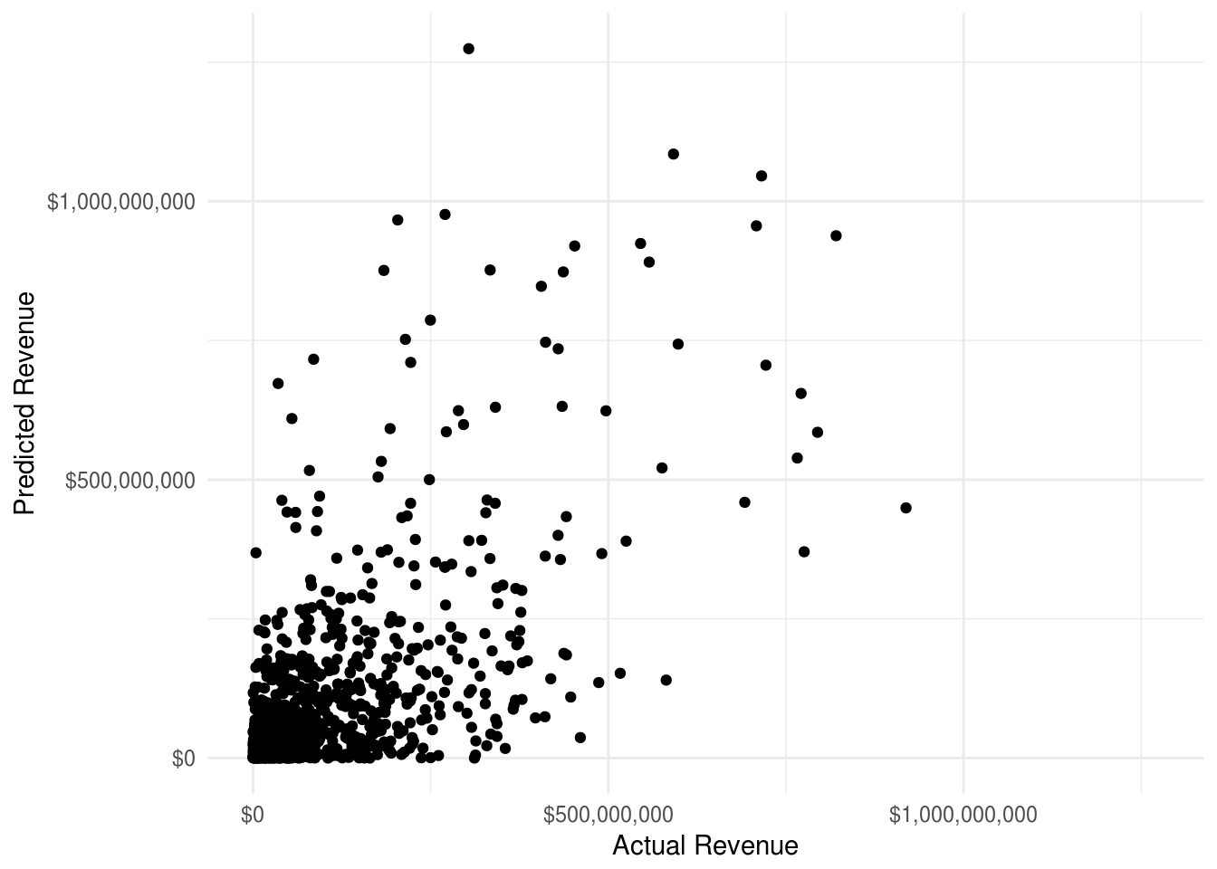
This model definitely seems to be decidedly mediocre, not great. Which, frankly, is to be expected given that we’re not taking into account the actual quality of the movie being made. Given that we’re only using plot summary, actors, genres, and production companies, and can still account for 33.2% of the variation is pretty impressive. This is also a good time to reflect on the utility of this kind of model, and the uncertainty baked in. If a production company were to use this model, it wouldn’t be best used as financial planning model, because it’s often off by some big margins. Rather, this model is most useful in establishing expectations for a given movie. Given the inputs available at the time, how well can we generally expect a movie to do. Movie execs may have reasons to believe a movie will do better or worse than it’s prediction, but at least this system provides an objective starting point for expectations.
Now that the model is built, let’s see what it expects for a movie potentially coming down the pipe. As many of you know, I’m LDS, and have many friends and family who are as well. One project I’ve seen come up on my social media feeds a lot is the Reign of Judges movie I linked to in the introduction. What this LDS filmmaker is doing is making a concept short, with the hopes of being picked up by a major production company. Obviously, the concerns I’ve talked as my motivation for building this model are valid here. The main thing the production company wants to know, is if this movie will make a lot of money or not. Well, they’ve posted a plot summary on their IMDB page, so we can use our model to estimate how it would do. What’s also cool about how the model is set up, is that we can assign different actors, and production companies to see what effect they would potentially have on the movie’s revenue.
First, let’s look at how the movie would do with no major actors (or rather, no actors who have been in 15 movies in the sample), and as an independent film with no major production company attached.
First we’ll read in the plot summary, and vectorize it.
##
  |
  |=================================================================| 100%
Next, let’s create the actor, genre, and production company columns.
## Actors (None Specified)
actors <- names(actor_valid)
zero <- rep(0, times=length(names(actor_valid)))
actors_base <- data.frame(t(zero))
names(actors_base) <- actors

## Production Company (None Specified)
pc <- names(pc_valid)
zero <- rep(0, times=length(names(pc_valid)))
pc_base <- data.frame(t(zero))
names(pc_base) <- pc

## Genre (War, Action, Drama Specified)
genre <- names(genre_valid)
zero <- rep(0, times=length(names(genre_valid)))
genre_base <- data.frame(t(zero))
names(genre_base) <- genre
genre_ <- c("Action", "War", "Drama")
genre_base[,genre_] <- 1
Now to combine all the features for this movie, and to score it.
tol_prepped <- cbind(dtm_tol, actors_base, genre_base, pc_base) %>%
  as.matrix()

empty <- predict(mod_revenue, tol_prepped)
empty
## [,1]
## [1,] 57538864The expected revenue is $57,538,864, which is the 0.4844082 of the movies in our sample. Not bad! But let’s see if we can’t get it higher by adding some big name actors and putting the movie at a major production company.
Now, I’m a human being who lives on earth, so I’m a big fan of Dwayne ‘The Rock’ Johnson. Let’s add him in the movie (he’d be a baller Captain Moroni). The intro to Vin Diesel’s xXx was filmed in my hometown, so I feel like I should add him in here as a shout-out.
Off the top of my head, it seems like Legendary Pictures would be a good fit for this movie, and since they have a deal with Universal right now, we’ll select those two companies.
## Actors (None Specified)
actors <- names(actor_valid)
zero <- rep(0, times=length(names(actor_valid)))
actors_base <- data.frame(t(zero))
names(actors_base) <- actors
actors <- c("DwayneJohnson", "VinDiesel")
actors_base[,actors] <- 1

## Production Company (None Specified)
pc <- names(pc_valid)
zero <- rep(0, times=length(names(pc_valid)))
pc_base <- data.frame(t(zero))
names(pc_base) <- pc
pc <- c("UniversalPictures", "LegendaryPictures")
pc_base[,pc] <- 1

## Genre (War, Action, Drama Specified)
genre <- names(genre_valid)
zero <- rep(0, times=length(names(genre_valid)))
genre_base <- data.frame(t(zero))
names(genre_base) <- genre
genre_ <- c("Action", "War", "Drama")
genre_base[,genre_] <- 1
tol_prepped <- cbind(dtm_tol, actors_base, genre_base, pc_base) %>%
as.matrix()
added <- predict(mod_revenue, tol_prepped)
added## [,1]
## [1,] 369004352So adding those features to the movie increased the revenue all the way up to $369,004,352, which would put the movie in the 91.9% percentile. That’s a big jump! Even though I woudn’t necessarily bet on it doing quite as well as this prediction, what I do think those model shows is that, if executed properly, this is an idea that has the potential to be big. Hopefully the concept short goes well, and some production company takes a bet on it and makes a bunch of money!
So there it is! We’ve built a model that does a decidedly ok job of predicting movie revenue with relatively few features. Hopefully this was a fun, educating, and entertaining read for you, because doing this analysis was quite a bit of fun for me.
This model was a lot of fun to create, and I there are some clear next steps I’m planning to take.
- There are still features to add that could increase the utility of this model. Specifically, adding directors, screenwriters, etc.
- The deep learning model can certainly use some more tuning. I’ve completed some trainings and done learning on my own, but I still recognize there’s a lot I still need to learn about this method.
- Having this model just live in R makes in useless for the vast majority of the population. I’m currently working on getting this into a Shiny app so all you weirdos can test out your movie ideas.
- This one is further down the pipeline, but it’d be fun to throw LIME at this problem to see which aspects of the movie are contributing and taking away from the movie realizing it’s fullest potential.
