
Case Study in Quantifying Risk and Reward with Tensorflow Probability
Building on what I was working on with my last post, where I was learning Tensorflow probability, I found that it was able to pick up the skew of simulated data pretty well, now I want to try it out on a real financial dataset.
For this, I picked the loan data from Lending Club. This is a nice dataset for this task because there’s a natural skew in the data due to defaults, where a borrower ends up paying less than the full amount they were lent. However, not all defaults are created equal, sometimes the borrow may end up paying 70% of the total loan, other times they may end up paying 10% of the total loan, and in some rare cases they’ll end up paying more than the amount loaned. For cases where the loan is fully paid, borrowers will pay the amount of the loan, plus some amount of interest.
When I’ve talked to people who invest with Lending Club, most of them take the approach of minimizing likelihood of default, whether though a classification algorithm, or by selecting only ‘A’ graded loans. (Alas, as I live in Ohio, the only state where you can’t fund or even buy loans, I have to take others’ words for it).
However, there may be an inefficiency with this approach. As with most things in finance, the more you risk, the more your potential reward. Loans with a higher risk of default will have higher interest rates, and depending on a number of factors, the borrower may have higher ability to pay than their grade reflects. It’s also important to differentiate between loans that are more likely to default at, say, 70% of the loan amount vs ones that are likely to default at 10% of the loan amount in order to determine whether the upside is worth the risk.
This is a case where I believe that modeling distributions is an improvement over a traditional regression or classification approach. Regression may not pick up the uncertainty around the prediction, especially since the distribution is skewed, and classification will ignore variation within classes, which can be a big deal. There are creative ways to deploy either type of algorithm that can circumvent these concerns (quantile regression, or multi-class problem at various thresholds of probability), but modeling the outcome distribution allows us to do all of these things within a single modeling framework.
Load Packages and Data
The data used for this analysis is the Lending Club loan data from 2007-2011, which can be accessed here or here
library(reticulate)
library(tictoc)
library(tensorflow)
library(tfprobability)
library(keras)
library(data.table)
library(dtplyr)
library(tidyverse)
library(recipes)
library(rsample)

dat <- fread('loan.csv') %>% as_tibble()


dat <- dat %>%
  filter(loan_status %in% c('Charged Off', 'Fully Paid'),
         application_type=='Individual') %>%
  mutate(pct_return=total_pymnt/funded_amnt)
Exploratory Data Analysis
First, let’s see the skew in percent of original loan payed back
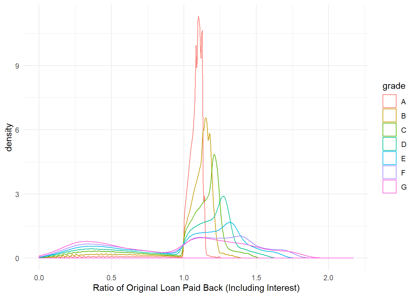
We see here what we’d expect. Grade A loans are highly concentrated slightly above 1, while as you go lower with grades, the proportion of this distribution above 1 moves to the right while the proportion of the distribution below 1 (defaults) increases as well. In other words, we see there that there’s more risk associated with more upside.
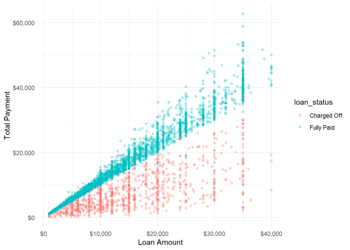
Now I’ll look at the total amount paid by the total amount funded to see the skew in a different way.
And looking at the same chart with ratio of return instead of raw return
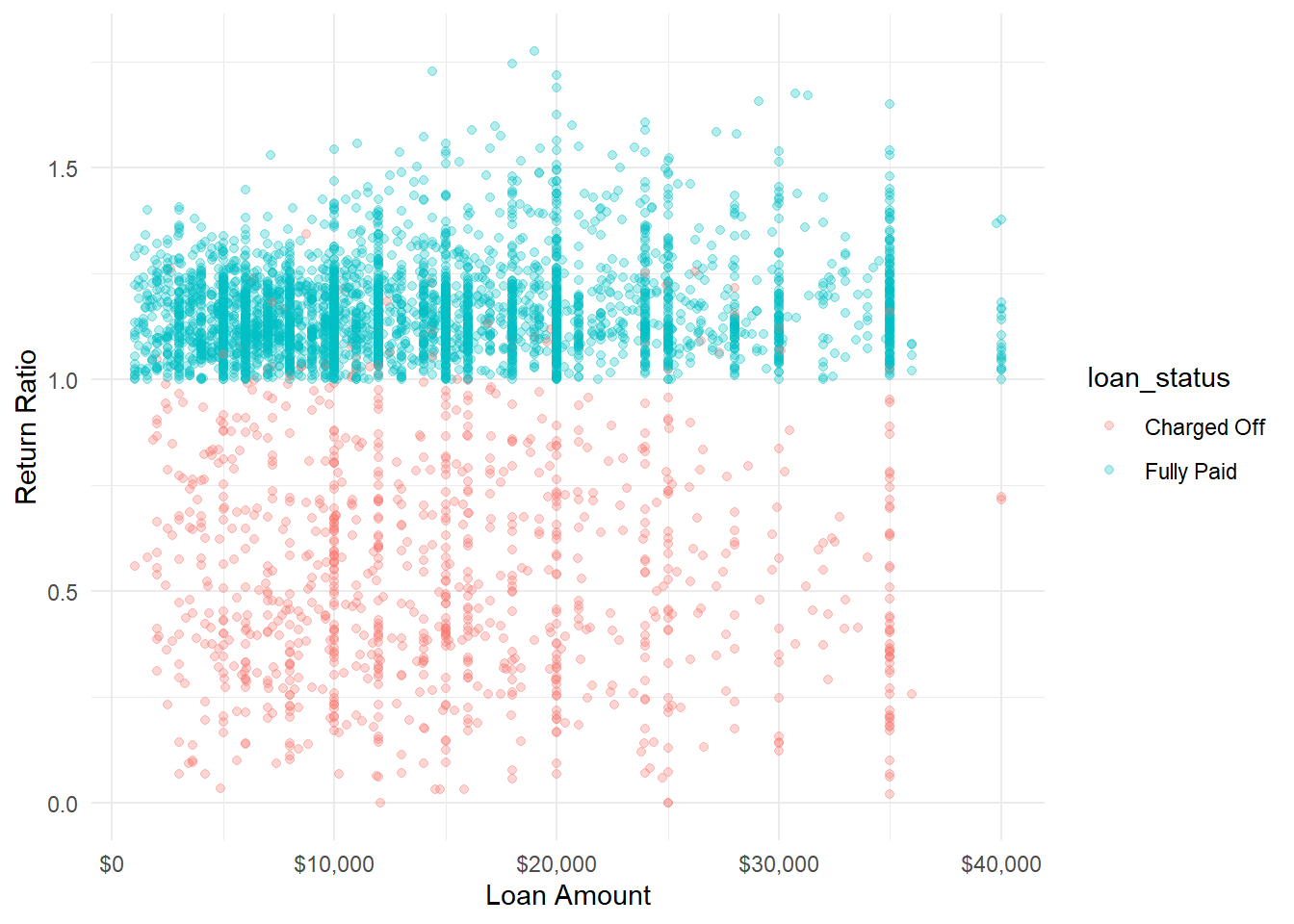
Either way you slice it, there’s definitely a skew in the data, a perfect problem for tfprobability!
Modeling Prep
To prepare the design matrix, I’ll use the recipes package, which allows me to automate my data cleaning steps to produce consistent design matrices. What I do here is log transform the annual income variable, discretize the inquiry and delinquency variables, scale and center numeric variables, and create dummy variables for categorical variables.
## Train/Test Split
split <- rsample::initial_split(dat, strata=pct_return)

## Data Prep
rec <- recipe(~ loan_amnt + int_rate + installment + sub_grade + purpose + annual_inc + home_ownership + inq_last_6mths + term + collections_12_mths_ex_med, data=training(split)) %>%
  step_mutate(inq_last_6mths = case_when(is.na(inq_last_6mths) ~ 'missing',
                                         inq_last_6mths>0 ~ 'mt1',
                                         TRUE ~ 'none'),
              collections_12_mths_ex_med = case_when(is.na(collections_12_mths_ex_med) ~ 'missing',
                                         inq_last_6mths>0 ~ 'mt1',
                                         TRUE ~ 'none')) %>%
  step_log(annual_inc, installment) %>%
  step_scale(all_numeric()) %>%
  step_center(all_numeric()) %>%
  step_other(all_nominal(), other = 'infreq', threshold = .01) %>%
  step_novel(all_nominal()) %>%
  step_dummy(all_nominal()) %>%
  step_zv(all_predictors())

prepped_rec <- prep(rec)

## Generate Input Matrices
x_train <- juice(prepped_rec) %>% as.matrix()
x_test <- bake(prepped_rec, testing(split)) %>% as.matrix()

## Extract Output Variable
y_train <- training(split) %>% .$pct_return
y_test <- testing(split) %>% .$pct_return
Modeling
In specifying the model, I ended up settling on a fairly large network. That’s been a theme I’ve seen as I work with these probability models, that larger-than-expected networks are needed to fit even simple models. And I’ll note here, too, that I didn’t see any over-fitting between the train and test data yet, so it may be appropriate to grow the network even bigger.
model <- keras_model_sequential() %>%
  layer_dense(units = 32, activation = "relu", regularizer_l2()) %>%
  layer_dense(units = 64, activation = "relu", regularizer_l2()) %>%
  layer_dense(units = 128, activation = "relu", regularizer_l2()) %>%
  layer_dense(units = 64, activation = "relu", regularizer_l2()) %>%
  layer_dense(units = 32, activation = "relu", regularizer_l2()) %>%
  layer_dense(units = 4, activation = "linear") %>%
  layer_distribution_lambda(function(x) {
    tfd_sinh_arcsinh(loc = x[, 1, drop = FALSE],
                     scale = 1e-3 + tf$math$softplus(x[, 2, drop = FALSE]),
                     skewness=x[, 3, drop=FALSE],
                     tailweight=1e-3 + tf$math$softplus(x[, 4, drop = FALSE])
                     )
  }
  )

negloglik <- function(y, model) - (model %>% tfd_log_prob(y))


learning_rate <- 0.01
model %>% compile(optimizer = optimizer_adam(lr = learning_rate), loss=negloglik)

history <- model %>% fit(x_train, y_train,
                         validation_data=list(x_test, y_test),
                         epochs = 500,
                         batch_size=15000,
 callbacks=list(callback_early_stopping(monitor='val_loss', patience = 20))
                        )
Prediction
With distributional models, I’m able to extract various information from the predicted distribution. In this case, I take the probability of breaking even, the probability of profiting 10%, the 10th percentile, the 50th percentile, and the 90th percentile. This showcases the flexibility of these kinds of models, I can look at probabilities of certain thresholds occurring, or I can take various percentiles and see expected what would be expected at that percentile.
pred_dist <- model(tf$constant(x_test))

out <- testing(split) %>%
  select(total_pymnt, funded_amnt, int_rate, grade, sub_grade, loan_status, pct_return)

out$loc <- pred_dist$loc %>% as.numeric()
out$scale <- pred_dist$scale %>% as.numeric()
out$skewness <- pred_dist$skewness %>% as.numeric()
out$tailweight <- pred_dist$tailweight %>% as.numeric()
out$breakeven <- pred_dist$cdf(1) %>% as.numeric()
out$profit10 <- pred_dist$cdf(1.1) %>% as.numeric()
out$p90 <- pred_dist$quantile(.9) %>% as.numeric()
out$p50 <- pred_dist$quantile(.5) %>% as.numeric()
out$p10 <- pred_dist$quantile(.1) %>% as.numeric()
out$range <- out$p90-out$p10
Evaluation
I see two main things to evaluate: First, is my model accurately able to capture the spread of the outcome? Seconds, by reducing the model to a single point, are higher expected values of breaking even associated with higher actual breaking even values?
In terms of capturing the spread of the distribution, I’ll look at the likelihood crossing certain thresholds. Basically, the actual return rate should go above the 50th percentile about 50% of the time.
mean(out$pct_return>out$p10)## [1] 0.8804406mean(out$pct_return>out$p50)## [1] 0.469843mean(out$pct_return>out$p90)## [1] 0.06119491And that’s close to what we see here! Actual returns cross the 10th percentile 88% of the time, cross the 50th percentile 47% of the time, and cross the 90th percentile 6% of the time.
Looking at distributions by grade, we see that the range of distribution changes dramatically by grade.
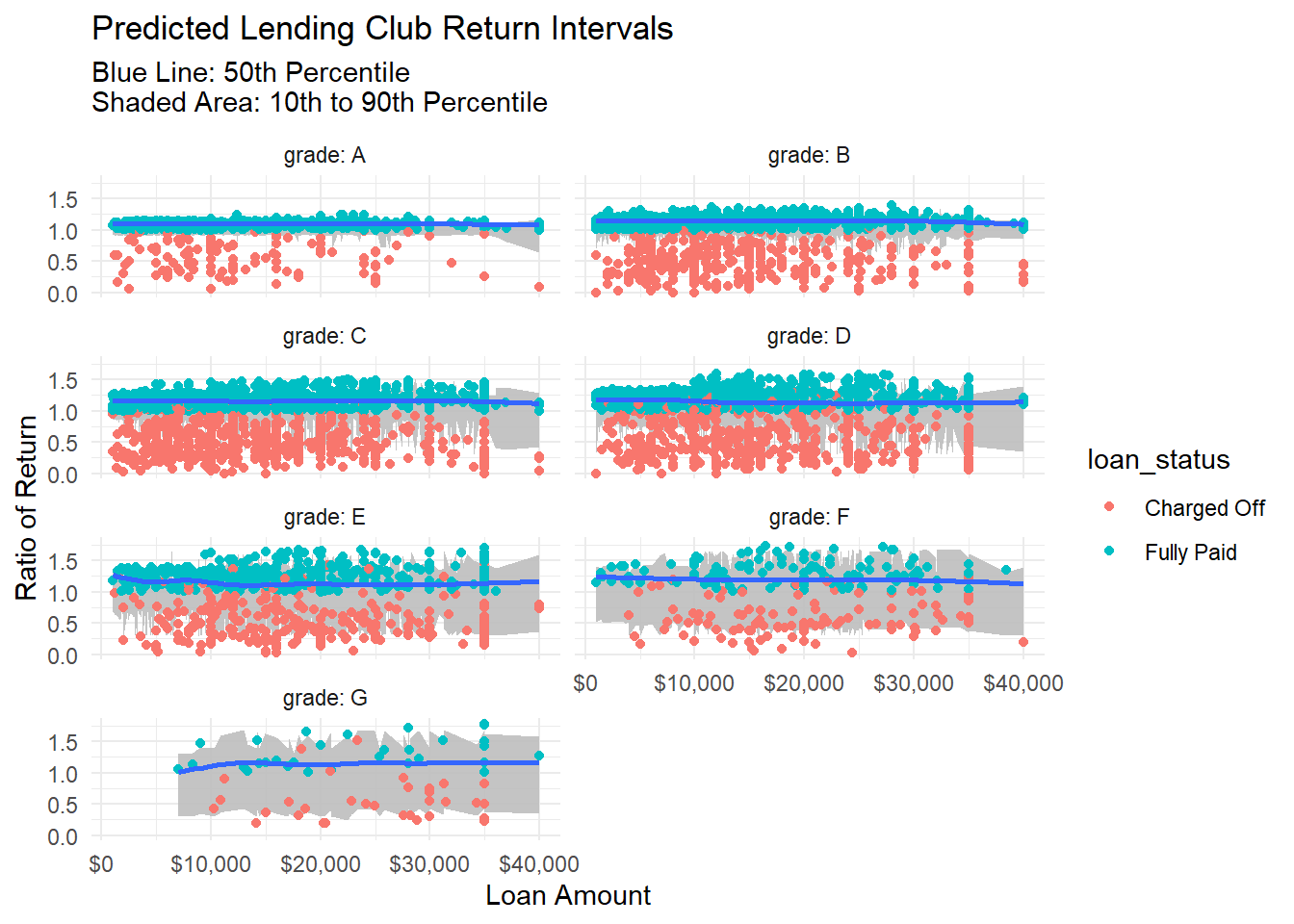
One note on the error distributions. You can see there’s a lot of noise there. This is due to the fact that I’m only plotting 2 dimensions (grade and loan amount), when I predicted with many more. For example, I’m not visually representing how income affects loans of certain grades at certain levels.
We can see the model picking up the spread and skew of the outcome by various grades, and the quantiles are doing a good job, but how are the cdf predictions doing? Do loans we predict have a higher likelihood of breaking even actually do so at a higher rate?
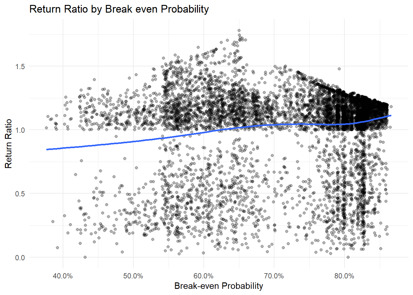
Overall, though there is a lot of noise here. I see the overall benefit of the model more so in accurately predicting the spread and shape of possible outcomes.
Conclusions
Distributional modeling allows us to look at problems in new ways, with greater information. With the case of Lending Club data, we can see how the spread of possible outcomes changes with various predictors, allowing investors to make better informed risk decisions. The model in this case is able to better predict the spread of return rather than exact return, but that may change with a more sophisticated model.
Some ways that the model may be improved are to use different underlying distributions. The T distribution comes to mind. However, I got worse performance with different ones, though that is probably more of a me problem than a ‘tfprobability’ problem. Another thing to keep in mind is that not all distributions have the same available extractions. For example, the `tfprobability’ module wouldn’t let me pull quantiles from the T distribution, and that’s a major feature I wanted. This might be moot, however, since the Sinh-Arcsinh transformation does so much distortion and transformation of the underlying distribution.
This post was not intended as investment advice.
