
Week 5 Fantasy Football Optimizations
We are BACK with optimal lineups from week 5 simulations!
I haven’t changed the script substantially since last week, and as I went over the code for scraping projections and generating lineups last week, I’ll skip some of that this week so we can focus more on the content. If you want to review it, the initial post is here.
Setup
library(data.table)
library(dtplyr)
library(tidyverse)
library(rPref)
library(kableExtra)

week <- 5

proj <- readRDS(paste0('week_', week, '_proj.RDS'))

sal <- read_csv(paste0('DKSalaries_wk_', week, '.csv'))
I’ll start with the optimized lineups pulled for week 4, with the same details as last time: 10,000 lineups, using the standard deviation of projections, completely individually based (still working on that).
sim_lu <- readRDS(paste0('sim_lineups_week_', week, '.RDS')) %>%
  rename(pts_base=points) %>%
  select(lineup, Name, team, position, pts_base, pts_pred, sd_pts, Salary)

glimpse(sim_lu)
## Observations: 90,000
## Variables: 8
## Groups: Name [148]
## $ lineup <int> 1, 1, 1, 1, 1, 1, 1, 1, 1, 2, 2, 2, 2, 2, 2, 2, 2, 2,...
## $ Name <chr> "Bengals", "Le'Veon Bell", "Zach Ertz", "Adam Thielen...
## $ team <chr> "CIN", "NYJ", "PHI", "MIN", "DAL", "DAL", "NOS", "CAR...
## $ position <chr> "DST", "RB", "TE", "WR", "WR", "QB", "WR", "RB", "WR"...
## $ pts_base <dbl> 7.186564, 17.660541, 14.598184, 16.137217, 4.449599, ...
## $ pts_pred <dbl> 8.122294, 20.390727, 18.380255, 20.284775, 11.993178,...
## $ sd_pts <dbl> 0.7662241, 1.8326980, 2.5496124, 2.0228734, 2.4638158...
## $ Salary <dbl> 2500, 6800, 6000, 6700, 3400, 6000, 6600, 8700, 3100,...sim_lu %>%
filter(lineup<=3) %>%
arrange(lineup, position, desc(pts_pred)) %>%
mutate_at(vars(pts_base, pts_pred, sd_pts), function(x) round(x, 2)) %>%
knitr::kable() %>%
kable_styling() %>%
column_spec(1, bold=TRUE) %>%
collapse_rows(columns = 1, valign = 'top') %>%
scroll_box(height = '500px', width = '100%')| lineup | Name | team | position | pts_base | pts_pred | sd_pts | Salary |
|---|---|---|---|---|---|---|---|
| 1 | Bengals | CIN | DST | 7.19 | 8.12 | 0.77 | 2500 |
| Dak Prescott | DAL | QB | 19.84 | 21.35 | 1.37 | 6000 | |
| Christian McCaffrey | CAR | RB | 24.04 | 23.58 | 0.91 | 8700 | |
| Le’Veon Bell | NYJ | RB | 17.66 | 20.39 | 1.83 | 6800 | |
| Zach Ertz | PHI | TE | 14.60 | 18.38 | 2.55 | 6000 | |
| Michael Thomas | NOS | WR | 18.58 | 23.33 | 2.31 | 6600 | |
| Adam Thielen | MIN | WR | 16.14 | 20.28 | 2.02 | 6700 | |
| Devin Smith | DAL | WR | 4.45 | 11.99 | 2.46 | 3400 | |
| Darius Slayton | NYG | WR | 2.69 | 11.10 | 2.48 | 3100 | |
| 2 | Buccaneers | TBB | DST | 6.46 | 6.65 | 0.35 | 2200 |
| Carson Wentz | PHI | QB | 20.64 | 22.70 | 1.25 | 6100 | |
| Christian McCaffrey | CAR | RB | 24.04 | 24.86 | 0.91 | 8700 | |
| David Johnson | ARI | RB | 20.06 | 22.34 | 1.95 | 7500 | |
| Chris Thompson | WAS | RB | 11.22 | 16.40 | 2.46 | 4600 | |
| Tyler Eifert | CIN | TE | 7.99 | 10.11 | 1.07 | 3300 | |
| DeAndre Hopkins | HOU | WR | 19.90 | 22.96 | 2.38 | 7800 | |
| Larry Fitzgerald | ARI | WR | 14.99 | 16.28 | 1.64 | 6000 | |
| Auden Tate | CIN | WR | 10.67 | 11.12 | 0.98 | 3500 | |
| 3 | Vikings | MIN | DST | 7.38 | 10.35 | 1.36 | 3200 |
| Dak Prescott | DAL | QB | 19.84 | 21.21 | 1.37 | 6000 | |
| Christian McCaffrey | CAR | RB | 24.04 | 25.13 | 0.91 | 8700 | |
| Leonard Fournette | JAC | RB | 18.01 | 20.21 | 1.25 | 6400 | |
| Aaron Jones | GBP | RB | 15.37 | 16.79 | 1.20 | 5900 | |
| Mark Andrews | BAL | TE | 11.72 | 15.14 | 2.89 | 4800 | |
| DeAndre Hopkins | HOU | WR | 19.90 | 22.64 | 2.38 | 7800 | |
| Auden Tate | CIN | WR | 10.67 | 11.80 | 0.98 | 3500 | |
| KeeSean Johnson | ARI | WR | 7.95 | 10.72 | 2.87 | 3500 |
Who is in Optimal Lineups?
sim_lu %>%
  group_by(Name, position, Salary) %>%
  dplyr::summarize(lu=n_distinct(lineup)) %>%
  ungroup() %>%
  group_by(position) %>%
  top_n(10, lu) %>%
  ungroup() %>%
  arrange(position, desc(lu)) %>%
  mutate(Name=factor(Name),
         Name=fct_reorder(Name, lu)) %>%
  ggplot(aes(x=Name, y=lu/1000, fill=Salary)) +
  geom_bar(stat='identity') +
  facet_wrap(~position, ncol = 3, scales='free') +
  coord_flip() +
  scale_y_continuous(labels = scales::comma) +
  scale_fill_viridis_c() +
  xlab('') +
  ylab('Lineups (Thousands)') +
ggtitle('Top 10 Players Present by Position') 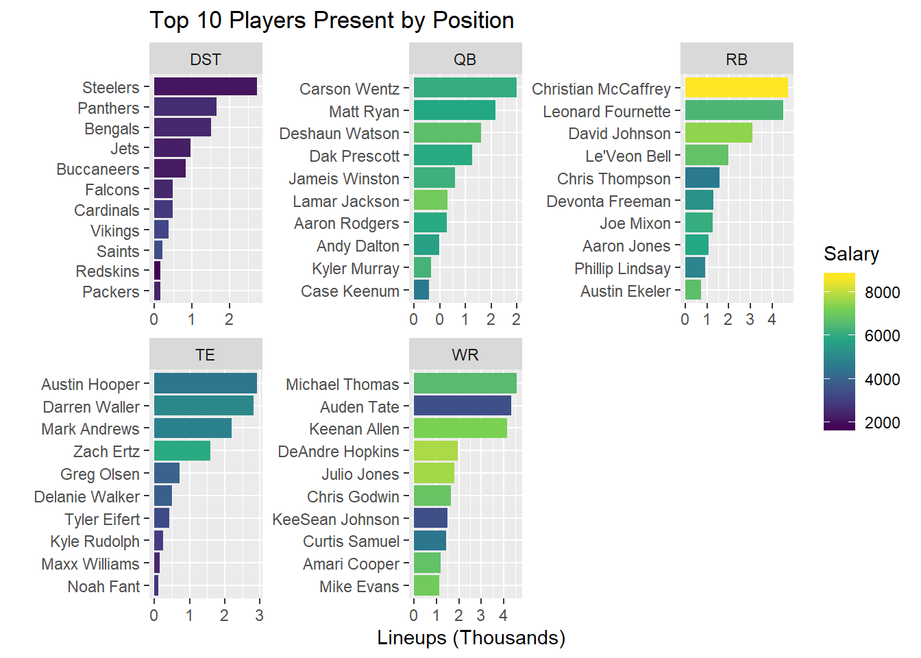
I’ve added a color dimension, which is the player’s salary, which helps us see if we’re adding studs at high prices, or more value selections. For example, Christian McCaffrey shows up a lot despite the high price, and Auden Tate shows up more due to his lower price.
Some of my observations:
Very flat week this week at the QB position with no QB showing up in more than 2,000 lineups. (Last week, Mahomes was in almost 6,000).
Christian McCaffrey and Leonard Fournette appear to be the favorites at RB, forming a kind of ‘Tier 1’ with David Johnson close behind.
Keenan Allen and Michael Thomas are your high end recievers, and Auden Tate is your big value play, at only $3,500 salary.
TE and D have similar patterns, there’s only 5 or so that you should really consider in your lineups.
Who is getting placed in Lineups?
DraftKings provides scoring for 416 players this week, but only 102 make it into optimized lineups. Why is that? To determine, I’ll plot projected points vs salary, colored by whether or not they make it into optimized lineups, and sized by their projection standard deviation
plyr_lu <- sim_lu %>%
  group_by(Name, position) %>%
  dplyr::summarize(lu=n_distinct(lineup)) %>%
  ungroup()

proj %>%
  filter(avg_type=='weighted') %>%
  mutate(Name = ifelse(pos=="DST", last_name, paste(first_name, last_name))) %>%
  inner_join(sal, by=c("Name")) %>%
  select(Name, team, position, points, Salary, sd_pts) %>%
  left_join(plyr_lu, by='Name') %>%
  replace_na(list(lu=0)) %>%
  mutate(lu_bin=ifelse(lu==0, '0 Lineups', '>=1 Lineups'),
         lu_5=cut(lu,5, labels = FALSE)) %>%
  ggplot(aes(x=Salary, y=points, color=lu_bin, size=sd_pts)) +
  geom_point() +
  scale_color_manual(values = c('red', 'blue'), name="") +
  geom_smooth(inherit.aes = FALSE, aes(x=Salary, y=points), method = 'lm', se=FALSE) +
  ylab('Projected Points') +
  xlab('Salary') +
  ggtitle('Who makes it into Optimized Lineups?') +
  scale_x_continuous(labels=scales::dollar)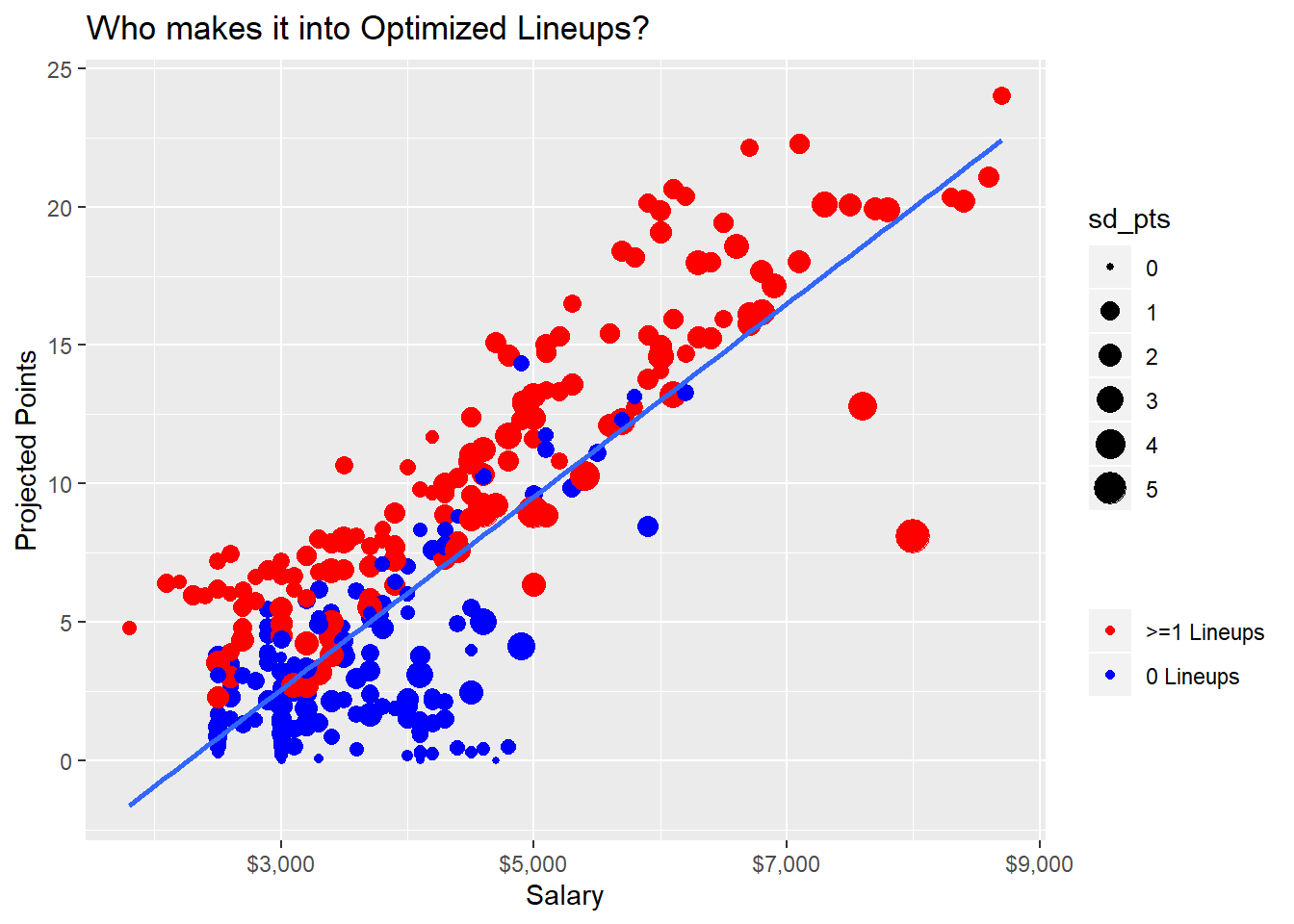
Interestingly, we see some players below the fitted line make it into optimal lineups, but we can see that these are due to high player uncertainty, so these are players with high potential to blow up, even though their average prediction is fairly low.
Flex Configurations
In DFS lineups, you have an extra spot to use on an RB, WR, and TE of your chosing
sim_lu %>%
  group_by(lineup) %>%
  mutate(lineup_pts=sum(pts_pred)) %>%
  group_by(lineup, position) %>%
  mutate(n=n()) %>%
  select(lineup, position, n, lineup_pts) %>%
  distinct() %>%
  spread(key=position, value=n) %>%
  filter(RB>=2, TE>=1, WR>=3) %>%
  mutate(flex=case_when(RB==3 ~ 'RB',
                        TE==2 ~ 'TE',
                        WR==4 ~ 'WR')) %>%
  group_by(flex) %>%
  dplyr::summarize(pts=median(lineup_pts),
                   cases=n()) %>%
  knitr::kable() %>%
kable_styling(full_width = FALSE)| flex | pts | cases |
|---|---|---|
| RB | 153.8310 | 3313 |
| TE | 155.0864 | 2043 |
| WR | 155.0120 | 4644 |
Again, WRs are the flex selection most of the time. Given what we saw with the last graph, this makes sense. There are some clear favorites in the WR spot that you’ll want to get, whereas RBs are fairly replaceable this week. And the situations where you want a TE in FLEX is when one really blows up, hence the higher average score.
Pareto Lineups
lu_df <- sim_lu %>%
  group_by(lineup) %>%
  dplyr::summarize(lineup_pts=sum(pts_pred),
                   lineup_sd=sum(sd_pts)) %>%
  ungroup()

pto <- psel(lu_df, low(lineup_sd) * high(lineup_pts))


ggplot(lu_df, aes(y=lineup_pts, x=lineup_sd)) +
  geom_point() +
  geom_point(data=pto, size=5) +
  ylab('Lineup Points') +
  xlab('Lineup Points St Dev') +
  ggtitle('Lineup Points vs Uncertainty',
          subtitle = 'Pareto Lineups Bolded')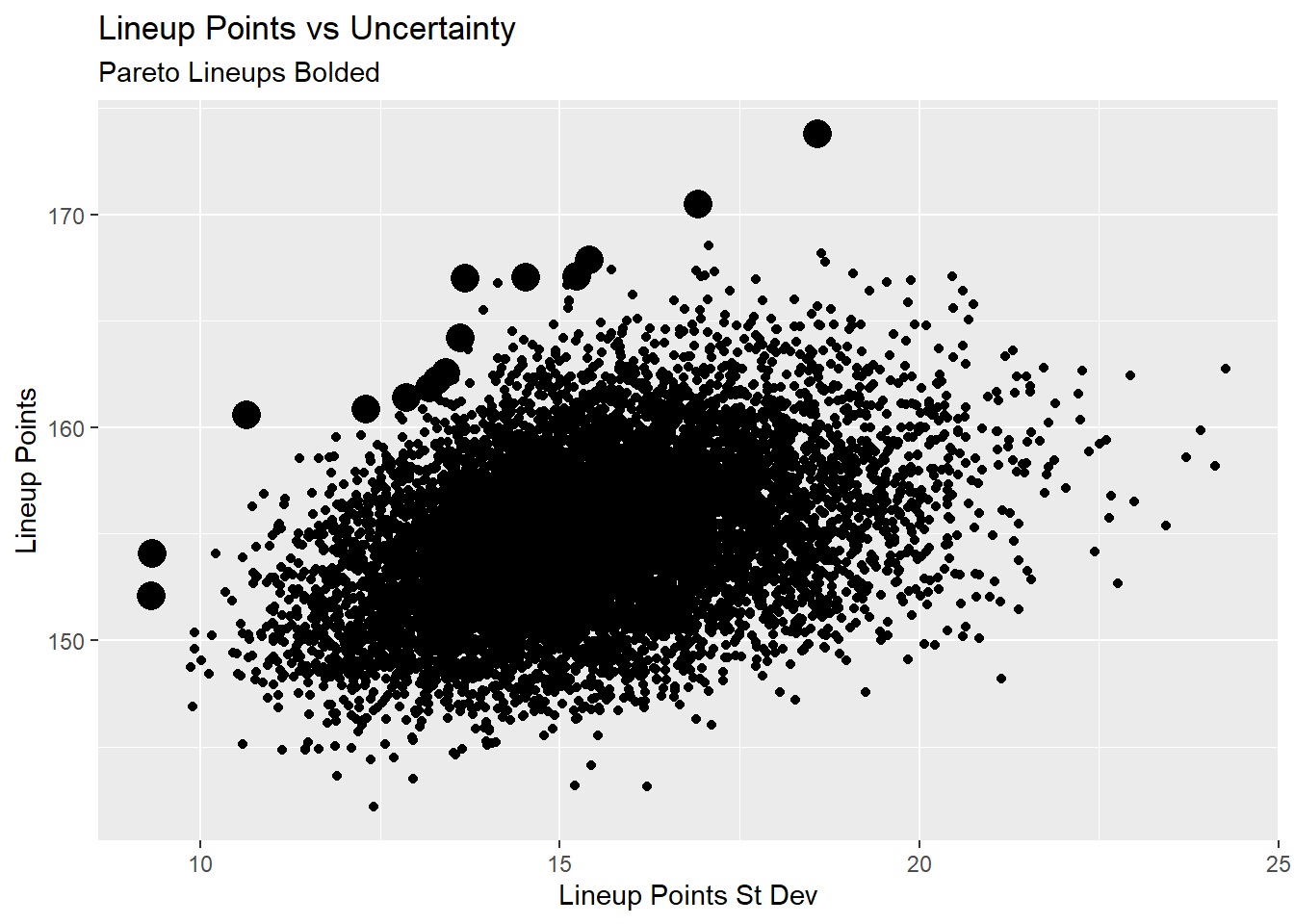
Here’s a look at the pareto lineups.
psel(lu_df, low(lineup_sd) * high(lineup_pts)) %>%
  left_join(sim_lu, by='lineup') %>%
  group_by(lineup) %>%
  arrange(lineup_pts, position, desc(pts_pred)) %>%
  select(lineup, lineup_pts, lineup_sd, Name, team, position, pts_pred, sd_pts, Salary) %>%
  mutate_at(vars(lineup_pts, lineup_sd, pts_pred, sd_pts), function(x) round(x, 2)) %>%
  knitr::kable() %>%
  kable_styling(fixed_thead = T) %>%
  column_spec(1:3, bold=TRUE) %>%
  collapse_rows(columns = 1:3, valign = 'top') %>%
scroll_box(height = '500px', width = '100%')| lineup | lineup_pts | lineup_sd | Name | team | position | pts_pred | sd_pts | Salary |
|---|---|---|---|---|---|---|---|---|
| 5249 | 152.08 | 9.32 | Panthers | CAR | DST | 8.94 | 0.84 | 2600 |
| Deshaun Watson | HOU | QB | 25.27 | 0.90 | 6700 | |||
| Christian McCaffrey | CAR | RB | 24.78 | 0.91 | 8700 | |||
| Alvin Kamara | NOS | RB | 23.59 | 1.42 | 8600 | |||
| Leonard Fournette | JAC | RB | 19.33 | 1.25 | 6400 | |||
| Tyler Eifert | CIN | TE | 9.33 | 1.07 | 3300 | |||
| Larry Fitzgerald | ARI | WR | 17.64 | 1.64 | 6000 | |||
| Mohamed Sanu | ATL | WR | 12.20 | 0.31 | 4200 | |||
| Auden Tate | CIN | WR | 10.98 | 0.98 | 3500 | |||
| 6462 | 154.08 | 9.33 | Panthers | CAR | DST | 9.64 | 0.84 | 2600 |
| Deshaun Watson | HOU | QB | 24.13 | 0.90 | 6700 | |||
| Christian McCaffrey | CAR | RB | 24.39 | 0.91 | 8700 | |||
| Leonard Fournette | JAC | RB | 19.58 | 1.25 | 6400 | |||
| Greg Olsen | CAR | TE | 11.47 | 0.59 | 4000 | |||
| Keenan Allen | LAC | WR | 24.30 | 2.56 | 7300 | |||
| Emmanuel Sanders | DEN | WR | 14.33 | 1.00 | 5100 | |||
| Courtland Sutton | DEN | WR | 14.31 | 0.99 | 4900 | |||
| Mohamed Sanu | ATL | WR | 11.93 | 0.31 | 4200 | |||
| 594 | 160.55 | 10.64 | Panthers | CAR | DST | 8.98 | 0.84 | 2600 |
| Deshaun Watson | HOU | QB | 24.76 | 0.90 | 6700 | |||
| Christian McCaffrey | CAR | RB | 25.56 | 0.91 | 8700 | |||
| Leonard Fournette | JAC | RB | 19.74 | 1.25 | 6400 | |||
| Greg Olsen | CAR | TE | 12.28 | 0.59 | 4000 | |||
| Keenan Allen | LAC | WR | 26.04 | 2.56 | 7300 | |||
| Michael Thomas | NOS | WR | 20.58 | 2.31 | 6600 | |||
| Mohamed Sanu | ATL | WR | 11.43 | 0.31 | 4200 | |||
| Auden Tate | CIN | WR | 11.18 | 0.98 | 3500 | |||
| 4191 | 160.84 | 12.30 | Falcons | ATL | DST | 7.38 | 1.11 | 2500 |
| Lamar Jackson | BAL | QB | 24.63 | 1.33 | 7100 | |||
| Christian McCaffrey | CAR | RB | 25.34 | 0.91 | 8700 | |||
| Leonard Fournette | JAC | RB | 20.17 | 1.25 | 6400 | |||
| Devonta Freeman | ATL | RB | 14.78 | 1.58 | 5300 | |||
| Darren Waller | OAK | TE | 21.01 | 2.27 | 5000 | |||
| Keenan Allen | LAC | WR | 24.43 | 2.56 | 7300 | |||
| Mohamed Sanu | ATL | WR | 12.19 | 0.31 | 4200 | |||
| Auden Tate | CIN | WR | 10.91 | 0.98 | 3500 | |||
| 1002 | 161.38 | 12.87 | Steelers | PIT | DST | 7.95 | 1.03 | 2100 |
| Carson Wentz | PHI | QB | 22.54 | 1.25 | 6100 | |||
| Christian McCaffrey | CAR | RB | 24.28 | 0.91 | 8700 | |||
| Leonard Fournette | JAC | RB | 19.19 | 1.25 | 6400 | |||
| Darren Waller | OAK | TE | 18.33 | 2.27 | 5000 | |||
| Keenan Allen | LAC | WR | 26.98 | 2.56 | 7300 | |||
| Michael Thomas | NOS | WR | 19.40 | 2.31 | 6600 | |||
| Mohamed Sanu | ATL | WR | 11.91 | 0.31 | 4200 | |||
| Auden Tate | CIN | WR | 10.80 | 0.98 | 3500 | |||
| 7012 | 161.86 | 13.19 | Steelers | PIT | DST | 7.82 | 1.03 | 2100 |
| Matt Ryan | ATL | QB | 20.70 | 1.02 | 5900 | |||
| Christian McCaffrey | CAR | RB | 24.03 | 0.91 | 8700 | |||
| Leonard Fournette | JAC | RB | 19.72 | 1.25 | 6400 | |||
| Austin Hooper | ATL | TE | 14.58 | 1.25 | 4500 | |||
| Michael Thomas | NOS | WR | 23.57 | 2.31 | 6600 | |||
| Larry Fitzgerald | ARI | WR | 18.91 | 1.64 | 6000 | |||
| Calvin Ridley | ATL | WR | 17.29 | 1.25 | 4900 | |||
| Curtis Samuel | CAR | WR | 15.24 | 2.54 | 4500 | |||
| 3347 | 162.22 | 13.29 | Panthers | CAR | DST | 8.52 | 0.84 | 2600 |
| Lamar Jackson | BAL | QB | 23.92 | 1.33 | 7100 | |||
| Christian McCaffrey | CAR | RB | 26.18 | 0.91 | 8700 | |||
| Aaron Jones | GBP | RB | 16.65 | 1.20 | 5900 | |||
| Zach Ertz | PHI | TE | 20.90 | 2.55 | 6000 | |||
| Michael Thomas | NOS | WR | 22.71 | 2.31 | 6600 | |||
| Robby Anderson | NYJ | WR | 15.52 | 1.92 | 4500 | |||
| Calvin Ridley | ATL | WR | 15.42 | 1.25 | 4900 | |||
| Auden Tate | CIN | WR | 12.39 | 0.98 | 3500 | |||
| 1021 | 162.56 | 13.41 | Panthers | CAR | DST | 7.83 | 0.84 | 2600 |
| Matt Ryan | ATL | QB | 21.04 | 1.02 | 5900 | |||
| Christian McCaffrey | CAR | RB | 25.42 | 0.91 | 8700 | |||
| Leonard Fournette | JAC | RB | 20.01 | 1.25 | 6400 | |||
| Darren Waller | OAK | TE | 17.44 | 2.27 | 5000 | |||
| Austin Hooper | ATL | TE | 15.11 | 1.25 | 4500 | |||
| Keenan Allen | LAC | WR | 26.79 | 2.56 | 7300 | |||
| Courtland Sutton | DEN | WR | 14.77 | 0.99 | 4900 | |||
| Nelson Agholor | PHI | WR | 14.14 | 2.35 | 4700 | |||
| 8620 | 164.19 | 13.62 | Redskins | WAS | DST | 5.52 | 0.36 | 1800 |
| Dak Prescott | DAL | QB | 21.56 | 1.37 | 6000 | |||
| Christian McCaffrey | CAR | RB | 25.31 | 0.91 | 8700 | |||
| Joe Mixon | CIN | RB | 20.25 | 1.26 | 6100 | |||
| Mark Andrews | BAL | TE | 17.85 | 2.89 | 4800 | |||
| Michael Thomas | NOS | WR | 23.97 | 2.31 | 6600 | |||
| Keenan Allen | LAC | WR | 23.96 | 2.56 | 7300 | |||
| Emmanuel Sanders | DEN | WR | 14.98 | 1.00 | 5100 | |||
| Auden Tate | CIN | WR | 10.81 | 0.98 | 3500 | |||
| 5278 | 167.00 | 13.68 | Redskins | WAS | DST | 5.32 | 0.36 | 1800 |
| Matt Ryan | ATL | QB | 20.39 | 1.02 | 5900 | |||
| David Johnson | ARI | RB | 24.22 | 1.95 | 7500 | |||
| Leonard Fournette | JAC | RB | 20.66 | 1.25 | 6400 | |||
| Zach Ertz | PHI | TE | 20.76 | 2.55 | 6000 | |||
| Austin Hooper | ATL | TE | 15.36 | 1.25 | 4500 | |||
| Keenan Allen | LAC | WR | 24.87 | 2.56 | 7300 | |||
| Mike Evans | TBB | WR | 23.14 | 1.78 | 7100 | |||
| Auden Tate | CIN | WR | 12.27 | 0.98 | 3500 | |||
| 9837 | 167.04 | 14.52 | Falcons | ATL | DST | 8.25 | 1.11 | 2500 |
| Matt Ryan | ATL | QB | 20.78 | 1.02 | 5900 | |||
| Christian McCaffrey | CAR | RB | 25.34 | 0.91 | 8700 | |||
| Leonard Fournette | JAC | RB | 20.30 | 1.25 | 6400 | |||
| Mark Andrews | BAL | TE | 20.70 | 2.89 | 4800 | |||
| Austin Hooper | ATL | TE | 14.98 | 1.25 | 4500 | |||
| Chris Godwin | TBB | WR | 25.04 | 2.48 | 6900 | |||
| Amari Cooper | DAL | WR | 19.06 | 2.66 | 6800 | |||
| Auden Tate | CIN | WR | 12.59 | 0.98 | 3500 | |||
| 2699 | 167.08 | 15.24 | Steelers | PIT | DST | 8.39 | 1.03 | 2100 |
| Teddy Bridgewater | NOS | QB | 18.38 | 1.32 | 5200 | |||
| Christian McCaffrey | CAR | RB | 25.33 | 0.91 | 8700 | |||
| Leonard Fournette | JAC | RB | 20.51 | 1.25 | 6400 | |||
| Devonta Freeman | ATL | RB | 16.27 | 1.58 | 5300 | |||
| Austin Hooper | ATL | TE | 13.43 | 1.25 | 4500 | |||
| Keenan Allen | LAC | WR | 28.62 | 2.56 | 7300 | |||
| Chris Godwin | TBB | WR | 21.09 | 2.48 | 6900 | |||
| KeeSean Johnson | ARI | WR | 15.06 | 2.87 | 3500 | |||
| 5758 | 167.84 | 15.41 | Steelers | PIT | DST | 7.29 | 1.03 | 2100 |
| Matt Ryan | ATL | QB | 20.50 | 1.02 | 5900 | |||
| Christian McCaffrey | CAR | RB | 25.21 | 0.91 | 8700 | |||
| Leonard Fournette | JAC | RB | 18.67 | 1.25 | 6400 | |||
| Mark Andrews | BAL | TE | 15.46 | 2.89 | 4800 | |||
| Keenan Allen | LAC | WR | 26.95 | 2.56 | 7300 | |||
| Julio Jones | ATL | WR | 23.59 | 1.92 | 7700 | |||
| KeeSean Johnson | ARI | WR | 17.78 | 2.87 | 3500 | |||
| Auden Tate | CIN | WR | 12.40 | 0.98 | 3500 | |||
| 1497 | 170.49 | 16.92 | Saints | NOS | DST | 10.77 | 1.21 | 3400 |
| Carson Wentz | PHI | QB | 22.94 | 1.25 | 6100 | |||
| Christian McCaffrey | CAR | RB | 22.89 | 0.91 | 8700 | |||
| Aaron Jones | GBP | RB | 17.20 | 1.20 | 5900 | |||
| David Montgomery | CHI | RB | 15.66 | 1.17 | 5200 | |||
| Mark Andrews | BAL | TE | 16.07 | 2.89 | 4800 | |||
| Michael Gallup | DAL | WR | 29.86 | 4.76 | 5000 | |||
| Keenan Allen | LAC | WR | 22.65 | 2.56 | 7300 | |||
| Auden Tate | CIN | WR | 12.45 | 0.98 | 3500 | |||
| 816 | 173.76 | 18.59 | Panthers | CAR | DST | 9.01 | 0.84 | 2600 |
| Deshaun Watson | HOU | QB | 23.67 | 0.90 | 6700 | |||
| Leonard Fournette | JAC | RB | 18.50 | 1.25 | 6400 | |||
| Joe Mixon | CIN | RB | 17.02 | 1.26 | 6100 | |||
| Darren Waller | OAK | TE | 17.41 | 2.27 | 5000 | |||
| Michael Gallup | DAL | WR | 25.44 | 4.76 | 5000 | |||
| Michael Thomas | NOS | WR | 23.39 | 2.31 | 6600 | |||
| Amari Cooper | DAL | WR | 21.62 | 2.66 | 6800 | |||
| Nelson Agholor | PHI | WR | 17.69 | 2.35 | 4700 |
